A Hero’s Journey to Deep Learning CodeBase
Best Practices for Deep Learning CodeBase Series – Part II-B
By Dan Malowany and Gal Hyams @ Allegro AI
As the state-of-the-art models keep changing, one needs to effectively write a modular machine learning codebase to support and sustain R&D machine and deep learning efforts for years. In our first blog of this series, we demonstrated how to write a readable and maintainable code that trains a Torchvision MaskRCNN model, harnessing Ignite’s framework. In our second post (part IIA), we detailed the fundamental differences between single-shot and two-shot detectors and why the single-shot approach is in the sweet spot of the speed/accuracy trade-off. So it’s only natural that in this post we glean how to leverage the modular nature of the MaskRCNN codebase and enable it to train both MaskRCNN and SSD models. Thanks to the modular nature of the codebase, only minimal changes are needed in the code.
Torchvision is a package that consists of popular datasets, model architectures, and common image transformations for computer vision. It contains, among others, a model-zoo of pre-trained models for image classification, object detection, person keypoint detection, semantic segmentation and instance segmentation models, ready for out-of-the-box use. This makes a PyTorch user’s life significantly easier as it shortens the time between an idea and a product. Or a research paper. Or a blog post.
Torchvision does not contain implementations of single-shot object detection models, such as this popular SSD. So, we added one: an SSD implementation based on a Torchvision model as a backbone for feature extraction. Since its release, many improvements have been constructed on the original SSD. However, we have focused on the original SSD meta-architecture for clarity and simplicity. Let’s deep dive into the logic and methods of the implementation. The full code is available on Github.
Constants: Start with Default Values
First, we put our flashlight on the code constants, which are the default input arguments to the SSD class constructor. These are the common values for a 512×512 input image, tailored to the PASCAL-VOC dataset. (In part III of this series, we demonstrate how to adjust these values to your own dataset)
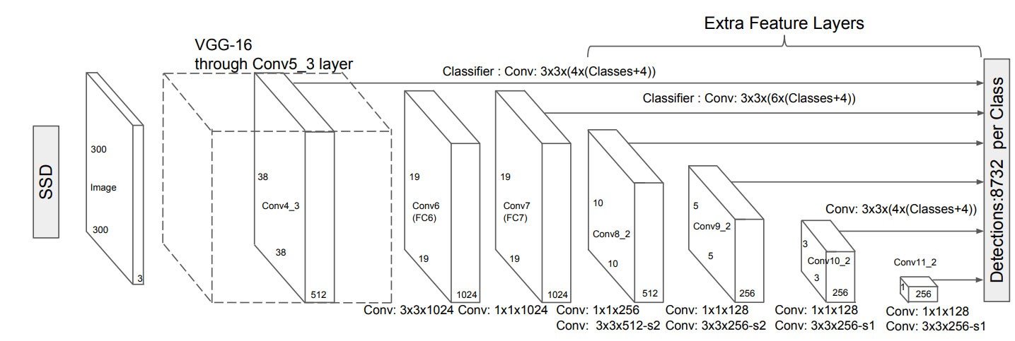
Each of these lists contains 7 entries – one entry per feature map from which object detection is done (see figure 1 above). Note that one of the lists, BOX_SIZES, has 8 entries and its computation is performed based on the entered values.
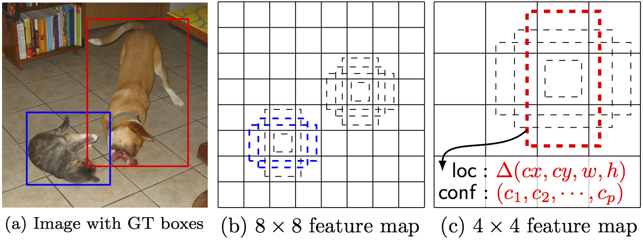
As illustrated in figure 2 (above), rectangle and square anchors tile the feature maps. The aspect_ratio list contains a list of rectangular aspect ratios for each feature map. Each number on this list defines two rectangles per prior center: one with the mentioned aspect ratio and one with it reversed. I.e, for each 2:1 ‘laying’ rectangle anchor, we have a 1:2 ‘standing’ rectangle anchor as well. In addition to the rectangular anchors, two sizes of square anchors are set over each prior center.
# The size ratio between the current layer and the original image.# I.e, how many pixel steps on the original image are equivalent to a single pixel step on the feature map.

STEPS = (8, 16, 32, 64, 128, 256, 512)

# Length of the shorter anchor rectangle face sizes, for each feature map.

BOX_SIZES = (35.84, 76.8, 153.6, 230.4, 307.2, 384.0, 460.8, 537.6)

# Aspect ratio of the rectangular SSD anchors, besides 1:1

ASPECT_RATIOS = ((2,), (2, 3), (2, 3), (2, 3), (2, 3), (2,), (2,))

# feature maps sizes.

FM_SIZES = (64, 32, 16, 8, 4, 2, 1)

# Amount of anchors for each feature map

NUM_ANCHORS = (4, 6, 6, 6, 6, 4, 4)

# Amount of each feature map channels, i.e third dimension.

IN_CHANNELS = (512, 1024, 512, 256, 256, 256, 256)
SSD Class Constructor
This SSD class produces an SSD object detection model based on Torchvision feature extractor, with the parameters described above.
class SSD(nn.Module):
   def __init__(self, backbone, num_classes, loss_function,

# Amount of anchors for each feature map
                num_anchors=NUM_ANCHORS,
                in_channels=IN_CHANNELS,
                steps=STEPS,
                box_sizes=BOX_SIZES,
                aspect_ratios=ASPECT_RATIOS,
                fm_sizes=FM_SIZES,
                heads_extractor_class=HeadsExtractor):

super(SSD, self).__init__()
...
self.extractor = heads_extractor_class(backbone)
self.criterion = loss_function
self.box_coder = SSDBoxCoder(self.steps, self.box_sizes, self.aspect_ratios, self.fm_sizes)

self._create_heads(
Create Classification and Localization Heads
Below, we first separate the feature maps’ decomposition from the SSD model in a way that lets you easily adapt the SSD to an adjusted feature maps’ extractor. If you do adapt the SSD, don’t forget to adapt the relevant parameters when calling the SSD constructor.
class HeadsExtractor(nn.Module):
   def __init__(self, backbone):
       super(HeadsExtractor, self).__init__()

       def split_backbone(net):
           features_extraction = [x for x in net.children()][:-2]

           if type(net) == torchvision.models.vgg.VGG:
               features_extraction = [*features_extraction[0]]
               net_till_conv4_3 = features_extraction[:-8]
               rest_of_net = features_extraction[-7:-1]
           elif type(net) == torchvision.models.resnet.ResNet:
               net_till_conv4_3 = features_extraction[:-2]
               rest_of_net = features_extraction[-2]
           else:
               raise ValueError('We only support VGG and ResNet backbones')
           return nn.Sequential(*net_till_conv4_3), nn.Sequential(*rest_of_net)

       self.till_conv4_3, self.till_conv5_3 = split_backbone(backbone)
       self.norm4 = L2Norm(512, 20)

       self.conv5_1 = nn.Conv2d(512, 512, kernel_size=3, padding=1, dilation=1)
       self.conv5_2 = nn.Conv2d(512, 512, kernel_size=3, padding=1, dilation=1)
       self.conv5_3 = nn.Conv2d(512, 512, kernel_size=3, padding=1, dilation=1)

       self.conv6 = nn.Conv2d(512, 1024, kernel_size=3, padding=6, dilation=6)
       self.conv7 = nn.Conv2d(1024, 1024, kernel_size=1)

       self.conv8_1 = nn.Conv2d(1024, 256, kernel_size=1)
       self.conv8_2 = nn.Conv2d(256, 512, kernel_size=3, padding=1, stride=2)

       self.conv9_1 = nn.Conv2d(512, 128, kernel_size=1)
       self.conv9_2 = nn.Conv2d(128, 256, kernel_size=3, padding=1, stride=2)

       self.conv10_1 = nn.Conv2d(256, 128, kernel_size=1)
       self.conv10_2 = nn.Conv2d(128, 256, kernel_size=3, padding=1, stride=2)

       self.conv11_1 = nn.Conv2d(256, 128, kernel_size=1)
       self.conv11_2 = nn.Conv2d(128, 256, kernel_size=3, padding=1, stride=2)

       self.conv12_1 = nn.Conv2d(256, 128, kernel_size=1)
       self.conv12_2 = nn.Conv2d(128, 256, kernel_size=4, padding=1
The SSD model shares all of the classification and localization computations, up until the final content classifier and spatial regressor. The create_heads method creates the SSD classification and localization heads on top of each feature map yielding per-anchor prediction. For each anchor, the localization head predicts a vector shifting and stretching (cx, xy, w, h), while the classification head predicts a vector of per-class probability.
   def _create_heads(self):
       self.loc_layers = nn.ModuleList()
       self.cls_layers = nn.ModuleList()
       for i in range(len(self.in_channels)):
       self.loc_layers += [nn.Conv2d(self.in_channels[i], self.num_anchors[i] * 4, kernel_size=3, padding=1)]
       self.cls_layers += [nn.Conv2d(self.in_channels[i], self.num_anchors[i] * self.num_classes, kernel_size=3, padding=1)]
The SSD model lays a hierarchy of feature maps, from the highest to the lowest resolution, and detects objects on each. The HeadsExtractor Class lays feature maps and makes them available for the detector. Its nomenclature is based on VGG-16 feature extractor (where conv4_3 is the name of the highest-resolution layer used as a feature map for the SSD model).
Different datasets and image sizes work best with an adjusted feature maps hierarchy; small images do not need as many different feature maps as large images do. Similarly, datasets without small objects can avoid high-resolution feature maps (accelerating the model computation time).
Define The SSD Forward Pass
In the following method, a forward pass of an image batch on the SSD model is calculated and its result is returned.
If the model is on evaluation mode, the forward pass returns the model prediction over the input image. However, if the forward pass is done in training mode, only the losses are returned. This is a common design that returns only the losses — which is more computationally efficient than returning all the detections.
With this method, the extracted_batch parameter holds the laid-out feature maps of the image batch, and then the prediction across each feature map is calculated separately.
   def forward(self, images, targets=None):
       if self.training and targets is None:
           raise ValueError("In training mode, targets should be passed")
       loc_preds = []
       cls_preds = []
       input_images = torch.stack(images) if isinstance(images, list) else images
       extracted_batch = self.extractor(input_images)
       for i, x in enumerate(extracted_batch):
           loc_pred = self.loc_layers[i](x)
           loc_pred = loc_pred.permute(0, 2, 3, 1).contiguous()
           loc_preds.append(loc_pred.view(loc_pred.size(0), -1, 4))

           cls_pred = self.cls_layers[i](x)
           cls_pred = cls_pred.permute(0, 2, 3, 1).contiguous()
           cls_preds.append(cls_pred.view(cls_pred.size(0), -1, self.num_classes))

       loc_preds = torch.cat(loc_preds, 1)
       cls_preds = torch.cat(cls_preds, 1)

      if self.training:
           encoded_targets = [self.box_coder.encode(target['boxes'], target['labels']) for target in targets]
           loc_targets = torch.stack([encoded_target[0] for encoded_target in encoded_targets])
           cls_targets = torch.stack([encoded_target[1] for encoded_target in encoded_targets])
           losses = self.criterion(loc_preds, loc_targets, cls_preds, cls_targets)
           return losses

       detections = []

       for batch, (loc, cls) in enumerate(zip(loc_preds.split(split_size=1, dim=0),

                                              cls_preds.split(split_size=1, dim=0))):

           boxes, labels, scores = self.box_coder.decode(loc.squeeze(), F.softmax(cls.squeeze(), dim=1))

           detections.append({'boxes': boxes, 'labels': labels, 'scores': scores})

       return detections
Connecting the SSD Model to CodeBase
To connect this code to the train & evaluation implementation using Ignite, we define
'model_type': 'ssd', 'ssd_backbone': 'resnet50',in the configuration data (manually or via Trains Server) and add the following code to the run method, which allows us to choose from among MaskRCNN, SSD meta-architectures, and the SSD backbone.
   # Get the relevant model based in task arguments

   if configuration_data.get('model_type') == 'maskrcnn':
       model = get_model_instance_segmentation(num_classes, configuration_data.get('mask_predictor_hidden_layer'))
   elif configuration_data.get('model_type') == 'ssd':
       backbone = get_backbone(configuration_data.get('backbone'))
       model = SSD(backbone=backbone, num_classes=num_classes, loss_function=SSDLoss(num_classes))
       model.dry_run(torch.rand(size=(1, 3, configuration_data.get('image_size'), configuration_data.get('image_size')))*255)
   else:
       raise ValueError('Only "maskrcnn" and "ssd" are supported as model type')
If you take a look at the train script you will see that besides the above configuration data changes, the only difference between the original MaskRCNN script and the new one, which support also SSD, is the model object definition section:
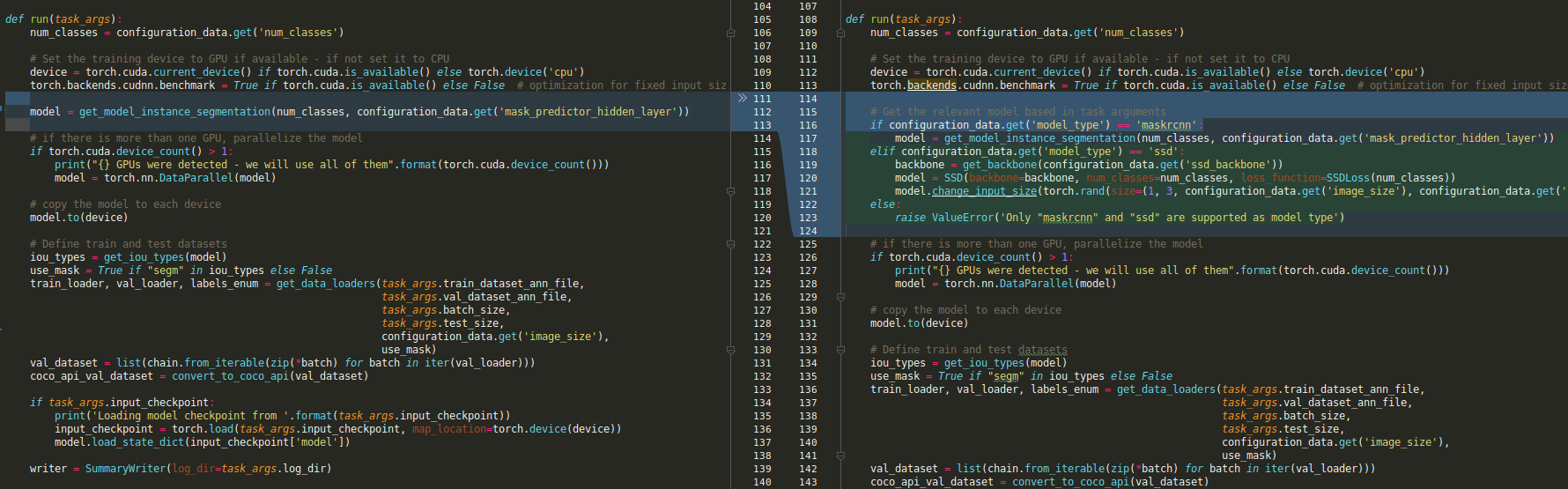
That means that all the rest of the assets in this codebase are kept unchanged. This is an enormous advantage from an R&D resources point of view.
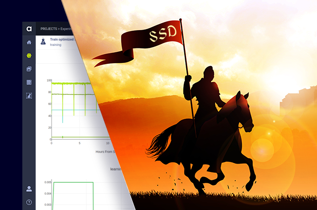
Allegro Trains – Sit Back, Relax & Monitor Your Experiment
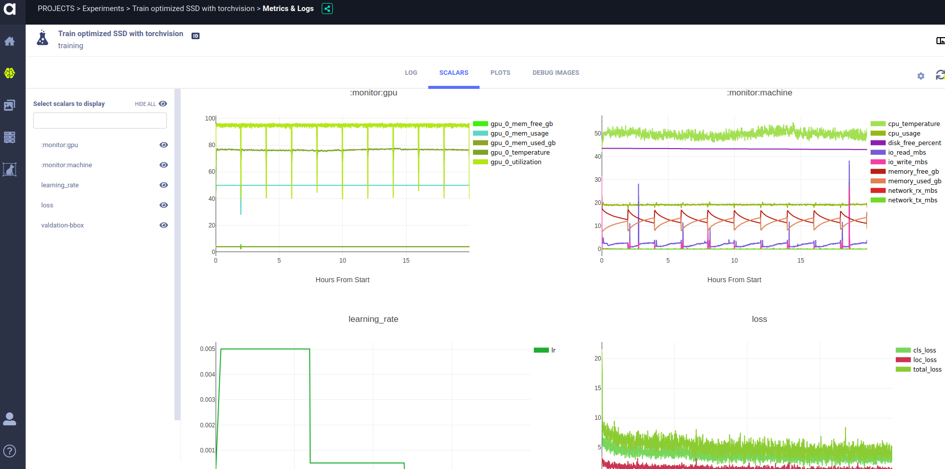
Allegro Trains, our open-source experiment & autoML manager, lets you easily monitor the model training process, including: statistics, such as real-time learning rate, loss, AUC and GPU monitoring, viewing debug-images to make sure all is well and comparing different experiments. All is logged into your own private Trains Server. In the snapshot above, we can see the progression of the learning rate and losses as the training progresses.
Conclusion
In the previous post (IIA), we reviewed in depth the advantages of single-shot detectors compared to two-shot. Here, we put this knowledge to code and create an SSD model on top of Torchvision, which you can use for your own purposes. In addition, we demonstrate the advantage of following this series’ guidelines of writing a maintainable and modular codebase.
The full code is available on Github. Parts of the SSD class presented here are based on this nicely written implementation of SSD. Thank you kuangliu 😉
In the next post, we show you how to optimize the SSD model and adjust it to your data. Stay tuned!